Impedance Matching with Parallel L and C

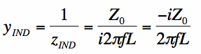
Parallel Inductors

The normalized admittance of an inductor y_ind is given by:

      [1]

Recall that if an admittance y_ind is placed in parallel with the load admittance y_L, the combination of the two admittances add. That is:

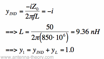
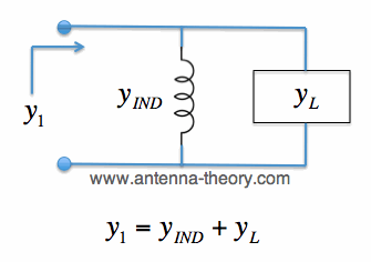Figure 1. Admittances in Parallel Add.

Since the admittance of an inductor is entirely imaginary (that is, Re[y_ind]=0), the result of adding an inductor in parallel is to change the susceptance of the antenna (load). That is, we are only altering the imaginary part of the antenna's admittance. Put another way, the result of a parallel inductor is to move the antenna impedance/admittance along the constant conductance circles.

As an example, suppose y_L = 1 + i*1. Then z_L= 0.5 - i*0.5

If we want to match the load (i.e., bring it to the center of the Smith Chart), then we want the parallel combination of the load (antenna) and the inductor to equal 1.0. Assuming Z0=50 Ohms and we are impedance matching at f=850 MHz, we can cancel out the susceptance of the load with a parallel inductor:

      [2]

The admittances y_1, y_L and y_IND are shown in Figure 2. Note the brown path shown. By using a parallel inductor, the antenna y_L can be moved counter-clockwise along the constant conductance circle Re[y]=1.0.

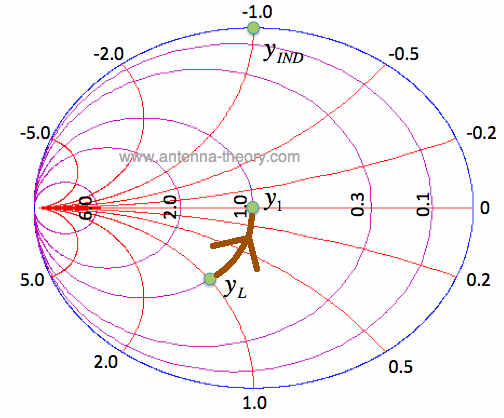Figure 2. Load Admittance Matched with using Parallel Inductor.

Parallel Capacitors

The normalized admittance of a capacitor y_C is given by:

      [3]

The capacitor in parallel with the load is shown in Figure 3.

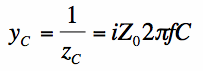
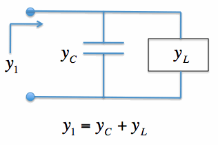Figure 3. Capacitor and Load in Parallel.

The effect of a parallel capacitor will be illustrated via an example. Suppose y_L= 0.3 - i*5. Then z_L = 0.012 + i*0.1993. To remove the susceptance from y_L, we can add in a capacitor with a susceptance of i*5. Assuming Z0=50 Ohms and f=2.4 GHz, we can calculate C:

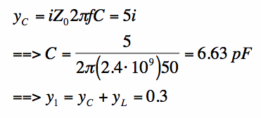      [4]

The admittances y_1, y_L and y_C are shown in Figure 4. Note the brown path shown. By using a parallel capacitor, the antenna y_L can be moved clockwise along the constant conductance circle Re[y]=0.3.

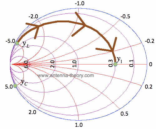Figure 4. Load Admittance Matched with using Parallel Capacitor.

Again, we can't perfectly match y_1 in this example with a parallel capacitor or inductor, because they only allow us to move along the constant susceptance curves. The point of this example is to understand how a parallel capacitor moves an admittance (load) on the Smith Chart.

To sum up this page: